")
JD
Calculating AD security metrics with BloodHound, Cypher, and a bit of graph analytics…
MATCH Blogpost = (:BloodHound)–[:Loves]->(:BlueTeam) RETURN Blogpost.Part1
I was working on some slides for my BloodHound workshop and while doing so, I was listening to a podcast where @_Wald0 (SpecterOps) talks about BloodHound, BloodHound Enterprise and AD metrics. And who better than Wald0 himself (co-creator of BloodHound alongside @CptJsesus & @harmj0y) to geek for an hour on how BloodHound can help defenders map attack paths and measure exposure in AD and AzureAD environments. If you want to know the WHYs and WHATs of Bloodhound metrics, this podcast is a great place to start.
Since the slides I was preparing were exactly on that topic, and since there is not much out there on HOW to do those type of BloodHound metrics calculations, I decided to write a post about it. That kind of Cypher post I wish I had found some time ago, when I started my adventures with BloodHound and Cypher in search for the perfect AD metric.
SPOILER: I still haven’t found that unicorn. But I’ve learned a few Cypher tricks on the way and I’ll happily share them with you if you like. Red or blue, I hope you’ll find it useful.

TL;DR: Calculating AD security metrics with BloodHound, Cypher, and graph analytics is really cool. And it’s even better when automated via the neo4j REST API. But I only have seeds – not fruits -, so you’re going to have to read on if you want to get the juice of it…
BloodHound was released in 2016 as a red team reconnaissance tool. But it’s 2023 by now and modern defenders are:
- Thinking in Graphs (see JohnLaTwc).
- Using BloodHound for AD/AAD security auditing (see cisa.gov).
- Using the Attack Path Management Methodology to reduce attack surface (see Wald0’s Manifesto).
- Tracking progress over time (in an Excel sheet mostly though… )
While BloodHound Enterprise was designed for blue teams and does all the above out-of-the-box for you, achieving the same kind of result in FOSS BloodHound can a bit more challenging. But if you are not afraid of Cypher (the neo4j database query language) and a bit of DIY, you can extract a lot of valuable metrics out of FOSS BloodHound. Even better: you can do it all in an automated way over the neo4j REST API.
Anti-virus products (and some security professionals) often consider BloodHound to be malware. 😦 This makes me sad… (and adds a folder exclusion to my box). Without diving into the OST debate, here’s my 2 cents on the topic (at least, for BloodHound):
- BloodHound itself has no “offensive” capability.
- BloodHound is just a UI and never touches the attacked network.
- SharpHound (the BloodHound data collector) is just a bunch of user-level LDAP queries. On steroids, maybe… but we can’t block automated LDAP queries or win32 API calls, right?
- PowerShell had the same bad reputation. Yet, PowerShell 💙 the Blue Team.
- Where I come from, we say “when you have a fever, there is no point in blaming the thermometer”.
Anyways, I hope by the end of this blog post you’ll be convinced: BloodHound 💙 the Blue Team.
Because a good graph speaks more than a 1000 words, BloodHound screenshots (or better: Export Graph > Export to PNG) are often used in reports to illustrate specific attack paths or visualize overall exposure to high-value assets. With a bit of extra mathematics, we can pimp those graphs by adding meaningful metrics next to them.
- Well-chosen graphs will help illustrating the situation you are describing.
- Well-chosen metrics will help understanding the graph you are displaying.
- Graphs are made to “get the (big) picture”.
- Metrics are here to quantify things.
This blog post will dive into exactly that: BloodHound Metrics.
So just hop in, and buckle up, if you want to join for the ride!

DISCLAIMER: I’m not a Cypher expert. I know nothing about graph analytics. If you are looking for an enterprise-grade solution, check out BloodHound Enterprise.
Show me the numbers
AD security is a complex beast. Adding AAD on top of that doesn’t make it easier. And beyond the obvious low-hanging fruits, looking at BloodHound graphs can get overwhelming quite quickly:
- What risks am I exposed to?
- How bad is it? Is it worse or better than last time / my neighbor ?
- How can I prioritize remediations?
- How can I translate that to upper management?
While numbers might not be the answer to everything, they can surely help answering some of our questions, since they are:
- Easy to grasp [understandable].
- Easy to share [communicable].
- Hard to deny [reproductible].
- Easy to track over time [comparable].
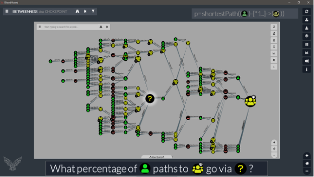
At the end of this post, you will be able to answer on the graph below. With only Cypher. For any graph. And for all nodes in the graph. In a single query.
This post is not about giving a list of queries, but more about explaining how it works, and I have sliced it as follows:
- Counting & Ranking
- Ratios & Percentages
- Out-Degree (aka “Reach”)
- In-Degree (aka “Exposure”)
- Betweenness (aka “Chokepoint”)
- REST API & automation
Topics 1 and 2 are covered in this first part of the blog. Topics 3-6 will be covered in a separate, second part of the blog.
NOTE: This post does not cover the offensive techniques associated to Bloodhound edges. If you are looking for documentation on that topic, check out the official BloodHound docs or this excellent ACL Hacker Recipe (by @_nwodtuhs). 👨🍳
Queries in this post are made to be run in the neo4j Browser/API and return metrics. If you are also looking for queries to return nodes/paths in the BloodHound UI, have a look at this (by Haus3c) or that (by mgeeky). You will probably find what you need in there, or at least some good inspiration to write you own custom queries.
Prior BloodHound & Cypher experience is probably required to fully enjoy this post. Links to the Neo4j Cypher Cheat Sheet are included throughout the post for quick syntax checks or links to the full Cypher reference manual.
All queries in this blog are generic and will work against your own AD. If you do not have access to AD, or want to practice with fake data, you can find a sample database here.
And so, after this (long) intro, let’s dive into this (long, long) blog post, and finally have a look at some Cypher.
1. Counting and ranking
When working in the BloodHound UI, counts of Nodes, Edges and Paths can be found in the DB Info tab & Node Info tab. Clicking on those numbers under the Node Info tab will display the matching graph (and show the Cypher query for that graph in the Query Input box, if you activate the Query Debug mode in the Settings dialog box).
Returning other (more complex) counts is not possible in the UI, as BloodHound was designed to return graphs or nodes. But for these kind of queries, we can use the neo4j browser located at http://localhost:7474 (replace localhost with the relevant IP for a remote DB).
Once in the neo4j browser, we can start counting objects. To do this, we simply use the COUNT() function.
Note: The new count{} subquery syntax (v5+) is not used in this post (but it looks really handy).
The basic Cypher syntax to count objects is as follows:
//// NODES
// Count all nodes.
MATCH (x) RETURN COUNT(x)
// Count Nodes of a specific type.
MATCH (u:User) RETURN COUNT(u)
// Count Nodes with a specific type and property.
MATCH (k:User {hasspn:true}) RETURN COUNT(k)
//// EDGES
// Count all Edges.
MATCH ()-[r]->()RETURN COUNT(r)
// Count Edges of a specific type.
MATCH ()-[r:AdminTo]->()RETURN COUNT(r)
// Count Edges with a specific property.
MATCH ()-[r {isacl:true}]->()RETURN COUNT(r)
The text output of these basic count queries looks like this in the neo4j browser:
╒══════════╕
│"COUNT(r)"│
╞══════════╡
│13636     │
└──────────┘
We can rename columns on the fly in the RETURN clause, using AS followed by the name we want to give it:
// Count all Edges.
MATCH ()-[r]->()
RETURN COUNT(r) AS EdgeCount
╒═══════════╕
│"EdgeCount"│
╞═══════════╡
│13636      │
└───────────┘
To group multiple counts into a single query, we can use the WITH clause to carry-over variables to the next part of our query. The WITH clause works like RETURN, except we can continue after:
// Count Nodes and Edges.
MATCH (x)
WITH COUNT(x) AS NodeCount
MATCH ()-[r]->()
RETURN NodeCount, COUNT(r) AS EdgeCount
╒═══════════╤═══════════╕
│"NodeCount"│"EdgeCount"│
╞═══════════╪═══════════╡
│1154       │13636      │
└───────────┴───────────┘
Adding another item to our counts could look something like this:
// Count Nodes, Edges and ACLs.
MATCH (x)WITH COUNT(x) AS NodeCount
MATCH ()-[r]->()WITH COUNT(r) AS EdgeCount,NodeCount
MATCH ()-[a {isacl:true}]->()
RETURN NodeCount, EdgeCount, COUNT(a) AS ACLCount
╒═══════════╤═══════════╤══════════╕
│"NodeCount"│"EdgeCount"│"ACLCount"│
╞═══════════╪═══════════╪══════════╡
│1154       │13636      │10573     │
└───────────┴───────────┴──────────┘
As you can imagine, adding another item would start to make it a painful construct…
To avoid having to use WITH to carry-over more and more variables after each MATCH we want to add to our query, we can also use sub-queries. This is done with the CALL {} syntax:
// Count Nodes, Edges and ACLs.
CALL {MATCH (x) RETURN COUNT(x) AS NodeCount}
CALL {MATCH ()-[r]->() RETURN COUNT(r) AS EdgeCount}
CALL {MATCH ()-[a {isacl:true}]->() RETURN COUNT(a) AS ACLCount}
RETURN NodeCount, EdgeCount, ACLCount
╒═══════════╤═══════════╤══════════╕
│"NodeCount"│"EdgeCount"│"ACLCount"│
╞═══════════╪═══════════╪══════════╡
│1154       │13636      │10573     │
└───────────┴───────────┴──────────┘
The output is the same, but the query is a bit easier to construct and read (imo).
With this technique, we could extract all the info from the DB Info Tab in a single query. But wait, with less typing involved, we can also use some Cypher functions to do the job…
To extract the type of a node (aka label), we can use the LABELS() function. So, we want to get those labels, group them by type and count them.
Count of Labels per Type:
// Return Count of Labels (Node Type).
MATCH (x)
WITH DISTINCT LABELS(x) AS Labels, COUNT(x) AS Count
RETURN Labels,Count
There is a bit more happening in this query, so let’s break it down:
- MATCH (x) is used to get all nodes.
- LABELS(x) is the neo4j function to extract labels from node x.
- WITH DISTINCT is used to “group by”.
- COUNT(x) after grouping, will count our nodes once grouped.
- and a RETURN clause to conclude as usual.
And this is what the output would look like:
╒════════════════════╤═══════╕
│"Label"             │"Count"│
╞════════════════════╪═══════╡
│["Base","Computer"] │519    │
├────────────────────┼───────┤
│["Base","Group"]    │70     │
├────────────────────┼───────┤
│["Base","User"]     │507    │
├────────────────────┼───────┤
│["Base","Container"]│24     │
├────────────────────┼───────┤
│["Base","Domain"]   │1      │
├────────────────────┼───────┤
│["Base","OU"]       │16     │
├────────────────────┼───────┤
│["Base","GPO"]      │17     │
└────────────────────┴───────┘
IMPORTANT: Nodes can have multiple labels (that’s why the function is called LABELS() with an ‘s’ at the end). In BloodHound, all nodes have a label “Base” and an “OtherLabel”. This OtherLabel is the one we are looking for most of the time (and the one that sets the icon for that node type).
To clean it up a bit and get rid of the “Base” label, we can simply index into the array:
// Return Count of labels (Node Type).
MATCH (x)
WITH DISTINCT LABELS(x)[1] AS Label, COUNT(x) AS Count
RETURN Label, Count
And if you don’t like indexing blindly into an array (just in case things are not always in the same position), you could do something more robust like this:
// Return Count of Labels (Node Type).
MATCH (x)
WITH DISTINCT [lbl IN LABELS(x) WHERE NOT lbl = 'Base'][0] AS Label, COUNT(x) AS Count
RETURN Label, Count
╒═══════════╤═══════╕
│"Label"    │"Count"│
╞═══════════╪═══════╡
│"Computer" │519    │
├───────────┼───────┤
│"Group"    │70     │
├───────────┼───────┤
│"User"     │507    │
├───────────┼───────┤
│"Container"│24     │
├───────────┼───────┤
│"Domain"   │1      │
├───────────┼───────┤
│"OU"       │16     │
├───────────┼───────┤
│"GPO"      │17     │
└───────────┴───────┘
Again, quite a lot happening in this short syntax (Cypher is really cool for that), so let’s have a closer look:
WITH DISTINCT [lbl IN LABELS(x) WHERE NOT lbl = 'Base'][0] AS Label
- LABELS(x) is used to extract labels of the nodes we are holding in x.
- lbl IN LABELS(x) is the way to name lbl the object we will iterate over it in next step.
- Then we add WHERE NOT lbl = ‘Base’ to filter out this ‘lbl’ we do not want.
The object we are holding at that point is an array containing one object, and since we know there is only one left in there, we can index safely into the array at position zero with [0] after the array.
- So the WITH DISTINCT creates a column holding a list of the unique types of edges excluding ‘Base’.
- Finally, we rename that column to ‘Label’ on the fly with AS.
Not too bad for a one-liner, right?
And you could, of course, use any other comparison operator than = within that construct (just like you would do when using WHERE after a MATCH) to extract the desired property if needed:
| # | Operator | Syntax | Example |
|---|---|---|---|
| Equals | = |
WHERE x.boolean = true |
|
| Not Equals | <> |
WHERE x.str <> 'Hello' |
|
| Greater Than | > |
WHERE x.num > 1 |
|
| Greater or Equal | >= |
WHERE x.num >= 1 |
|
| Less Than | < |
WHERE x.num < 1 |
|
| Less or Equal | <= |
WHERE x.num <= 1 |
|
| Exists | IS NOT NULL |
WHERE x.prop IS NOT NULL |
|
| Doesn’t Exist | IS NULL |
WHERE x.prop IS NULL |
|
| * | Starts with | STARTS WITH |
WHERE x.name STARTS WITH 'Alice' |
| * | Contains | CONTAINS |
WHERE x.name CONTAINS 'SQL' |
| * | Ends with | ENDS WITH |
WHERE x.objectid ENDS WITH '-512' |
| * | Regex | =~ |
WHERE x.name =~ '(?i).*adMiN.*' |
| Negate | NOT |
Negate any of the above: WHERE NOT x ... |
Operators marked with a * are string-specific.
With the same logic as in the previous query, we can use the TYPE() function on Edge objects to extract their type. Note how there is no ‘S’ here. That’s because edges can only have one type.
To extract and count all type of Edges:
// Count of Edges per type.
MATCH ()-[r]->()
WITH DISTINCT TYPE(r) AS Edge, COUNT(r) AS Count
RETURN Edge, Count
╒═════════════════════════╤═══════╕
│"Edge"                   │"Count"│
╞═════════════════════════╪═══════╡
│"Owns"                   │1344   │
├─────────────────────────┼───────┤
│"GenericAll"             │3294   │
├─────────────────────────┼───────┤
│"AddKeyCredentialLink"   │2046   │
├─────────────────────────┼───────┤
│"WriteDacl"              │1207   │
├─────────────────────────┼───────┤
│"WriteOwner"             │1207   │
├─────────────────────────┼───────┤
│"GenericWrite"           │1151   │
├─────────────────────────┼───────┤
│"MemberOf"               │1063   │
├─────────────────────────┼───────┤
│"AllExtendedRights"      │512    │
├─────────────────────────┼───────┤
│"Contains"               │1083   │
├─────────────────────────┼───────┤
│"GetChanges"             │3      │
├─────────────────────────┼───────┤
│"GetChangesInFilteredSet"│2      │
├─────────────────────────┼───────┤
│"GetChangesAll"          │2      │
├─────────────────────────┼───────┤
│"GPLink"                 │17     │
├─────────────────────────┼───────┤
│"DCSync"                 │5      │
├─────────────────────────┼───────┤
│"HasSession"             │700    │
└─────────────────────────┴───────┘
We could order edges alphabetically by adding an ORDER BY clause after the RETURN part of our query:
MATCH ()-[r]->()
WITH DISTINCT TYPE(r) AS Edge, COUNT(r) AS Count
RETURN Edge, Count
ORDER BY Edge
But since this post is mostly about numbers, we will use ORDER BY count DESCENDING to do just that:
MATCH ()-[r]->()
WITH DISTINCT TYPE(r) AS Edge, COUNT(r) AS Count
RETURN Edge, Count
ORDER BY Count DESCENDING
╒═════════════════════════╤═══════╕
│"Edge"                   │"Count"│
╞═════════════════════════╪═══════╡
│"GenericAll"             │3294   │
├─────────────────────────┼───────┤
│"AddKeyCredentialLink"   │2046   │
├─────────────────────────┼───────┤
│"Owns"                   │1344   │
├─────────────────────────┼───────┤
│"WriteDacl"              │1207   │
├─────────────────────────┼───────┤
│"WriteOwner"             │1207   │
├─────────────────────────┼───────┤
│"GenericWrite"           │1151   │
├─────────────────────────┼───────┤
│"Contains"               │1083   │
├─────────────────────────┼───────┤
│"MemberOf"               │1063   │
├─────────────────────────┼───────┤
│"HasSession"             │700    │
├─────────────────────────┼───────┤
│"AllExtendedRights"      │512    │
├─────────────────────────┼───────┤
│"GPLink"                 │17     │
├─────────────────────────┼───────┤
│"DCSync"                 │5      │
├─────────────────────────┼───────┤
│"GetChanges"             │3      │
├─────────────────────────┼───────┤
│"GetChangesInFilteredSet"│2      │
├─────────────────────────┼───────┤
│"GetChangesAll"          │2      │
└─────────────────────────┴───────┘
After ORDER BY count DESC, we add a final LIMIT clause, and we now get some rankings:
For example: the top 10 Computers with the most Sessions:
// Top 10 Computers with most Sessions.
MATCH (c:Computer)-[:HasSession]->(u:User)
WITH DISTINCT c.name AS Computer,COUNT(u) AS SessionCount
RETURN Computer, SessionCount
ORDER BY SessionCount DESCENDING
LIMIT 10
╒═══════════════════════╤══════════════╕
│"Computer"             │"SessionCount"│
╞═══════════════════════╪══════════════╡
│"PC0004.WHISPERER.LABZ"│5             │
├───────────────────────┼──────────────┤
│"PC0358.WHISPERER.LABZ"│5             │
├───────────────────────┼──────────────┤
│"PC0197.WHISPERER.LABZ"│4             │
├───────────────────────┼──────────────┤
│"PC0055.WHISPERER.LABZ"│4             │
├───────────────────────┼──────────────┤
│"PC0412.WHISPERER.LABZ"│4             │
├───────────────────────┼──────────────┤
│"PC0130.WHISPERER.LABZ"│4             │
├───────────────────────┼──────────────┤
│"PC0268.WHISPERER.LABZ"│3             │
├───────────────────────┼──────────────┤
│"PC0147.WHISPERER.LABZ"│3             │
├───────────────────────┼──────────────┤
│"PC0145.WHISPERER.LABZ"│2             │
├───────────────────────┼──────────────┤
│"PC0262.WHISPERER.LABZ"│2             │
└───────────────────────┴──────────────┘
Or, if we twist the query around a tiny bit: the top 10 Users with the most Sessions:
// Top 10 Users with the most Sessions.
MATCH (c:Computer)-[:HasSession]->(u:User)
WITH DISTINCT u.name AS User, COUNT(c) AS SessionCount
RETURN User, SessionCount
ORDER BY SessionCount DESCENDING
LIMIT 10
╒═════════════════════════════════╤══════════════╕
│"User"                           │"SessionCount"│
╞═════════════════════════════════╪══════════════╡
│"[email protected]"   │5             │
├─────────────────────────────────┼──────────────┤
│"[email protected]"  │5             │
├─────────────────────────────────┼──────────────┤
│"[email protected]"│5             │
├─────────────────────────────────┼──────────────┤
│"[email protected]"    │5             │
├─────────────────────────────────┼──────────────┤
│"[email protected]"   │5             │
├─────────────────────────────────┼──────────────┤
│"[email protected]"   │5             │
├─────────────────────────────────┼──────────────┤
│"[email protected]"   │4             │
├─────────────────────────────────┼──────────────┤
│"[email protected]"        │4             │
├─────────────────────────────────┼──────────────┤
│"[email protected]"   │4             │
├─────────────────────────────────┼──────────────┤
│"[email protected]"   │4             │
└─────────────────────────────────┴──────────────┘
Another example for this could be to get the Users with the most Group memberships:
// Top 5 Users with the most Group memberships.
MATCH (x)-[:MemberOf*1..]->(y)
WITH x.name AS Name, COUNT(y) AS MembershipCount
RETURN Name, MembershipCount
ORDER BY MembershipCount DESC
LIMIT 5
╒════════════════════════════════╤═════════════════╕
│"Name"                          │"MembershipCount"│
╞════════════════════════════════╪═════════════════╡
│"[email protected]"  │17               │
├────────────────────────────────┼─────────────────┤
│"[email protected]"         │7                │
├────────────────────────────────┼─────────────────┤
│"[email protected]" │7                │
├────────────────────────────────┼─────────────────┤
│"[email protected]"│7                │
├────────────────────────────────┼─────────────────┤
│"[email protected]" │6                │
└────────────────────────────────┴─────────────────┘
I guess you are starting the get the idea. The only point I want to make here is that we can, of course, count ‘chains’ of edges. In our last example of nested group memberships, simply by allowing multiple edges with the *1.. after the edge type (one or more MemberOf).
To be complete on specifying path length (aka the number of hops):
| Notation | Number of hops |
|---|---|
-[*1]-> |
One. |
-[]-> |
One. |
--> |
One. |
-[*2]-> |
Two. |
-[*0..]-> |
Zero or more… |
-[*1..]-> |
One or more… |
-[*]-> |
One or more… |
-[*1..4]-> |
One to Four. |
-[*2..5]-> |
Two to Five. |
And for specifying type of edges allowed:
| # | Syntax | Means |
|---|---|---|
-[:A]-> |
Edge A – One time | |
-[:A*1..]-> |
Edge A – One or more | |
-[:A|B]-> |
A OR B – One time | |
-[:A|B*1..]-> |
A OR B – One or more | |
| * | -[:!A]-> |
NOT A – One time |
| * | -[:!A*1..]-> |
NOT A – One or more |
| * | -[:(!A&!B)*1..]-> |
NOT A & NOT B – One time |
| * | -[:(!A&!B)*1..]-> |
NOT A & NOT B – One or more |
| ** | -[:{}*1..]-> |
UI Edge Filter – One or more |
* Only available in neo4j v5+. In v5, this ! notation can also be used to negate node labels… really cool stuff (check this & scroll up a tiny bit).
** Only works in BloodHound UI. The {} part will be replaced by whatever you have in your Edge filter when you run the query in the UI. It works like a charm, except for GPLink that you can’t get rid of – but that’s just a bug.
NOTE: At the time of writing of this post, the BloodHound documentation recommends using the latest v4, as it seems there are some issues with v5. I did some testing on my side of v5 and it seems ok so far, I have to say. But I haven’t really submitted it to heavy loads.
While we are here recapping some general Cypher syntax, let’s take a look at Date & Time.
// Current date.
RETURN date()
╒════════════╕
│"Today"     │
╞════════════╡
│"2023-03-23"│
└────────────┘
// Current time.
RETURN time() AS Now
╒═════════════════════╕
│"Now"                │
╞═════════════════════╡
│"19:31:49.409000000Z"│
└─────────────────────┘
// Current date and time.
RETURN datetime() AS FullDate
╒════════════════════════════════╕
│"FullDate"                      │
╞════════════════════════════════╡
│"2023-03-26T19:39:16.198000000Z"│
└────────────────────────────────┘
// Specific date.
RETURN datetime('2023-04-20T13:37:24.365+0100') AS ThatDate
╒═════════════════════════════════════╕
│"ThatDate"                           │
╞═════════════════════════════════════╡
│"2023-04-20T13:37:24.365000000+01:00"│
└─────────────────────────────────────┘
IMPORTANT: In the BloodHound UI, dates are displayed in human-readable format. However, they are stored in epoch format under the hood, so we must always use the epoch format in our queries. Used for: pwdlastset,lastlogon,lastlogontimestamp,whencreated.
Epoch basics:
// Date to epoch (now).
RETURN datetime().epochseconds AS Epoch
// Alternative.RETURN timestamp()/1000 AS Epoch
╒══════════╕
│"Epoch"   │
╞══════════╡
│1679860445│
└──────────┘
// Date to epoch (specific date).
RETURN datetime('2023-04-20T13:37:24.365+0100').epochSeconds AS ThatEpoch
╒═══════════╕
│"ThatEpoch"│
╞═══════════╡
│1681994244 │
└───────────┘
// Epoch to date.
RETURN datetime({epochseconds:1679860033}) AS DateTime
╒══════════════════════╕
│"DateTime"            │
╞══════════════════════╡
│"2023-03-26T19:47:13Z"│
└──────────────────────┘
So, if we wanted to do 90 days ago in epoch, we could do something like this:
// Epoch: 90 days ago (90x24hx60m*60s).
RETURN datetime().epochseconds - (90*24*60*60) AS Ago90
╒══════════╕
│"Ago90"   │
╞══════════╡
│1672089278│
└──────────┘
Or we could also use the duration() function:
// Epoch: 90 days ago.
RETURN (datetime()-duration({days:90})).epochseconds AS Ago90
╒══════════╕
│"Ago90"   │
╞══════════╡
│1672085576│
└──────────┘
// Epoch: 90 days ago at 00:00.
RETURN (datetime({date:date()})-duration({days:90})).epochseconds AS Ago90
╒══════════╕
│"Ago90"   │
╞══════════╡
│1672012800│
└──────────┘
To put this in practice, let’s return the count of passwords last set more than 90 days ago:
// PwdLastSet more than 90 days ago.
WITH 90 AS limit
MATCH (x:User) WHERE x.pwdlastset < (datetime()-duration({days:limit})).epochseconds
RETURN limit AS OlderThan, COUNT(x) AS Count
╒═══════════╤═══════╕
│"OlderThan"│"Count"│
╞═══════════╪═══════╡
│90         │414    │
└───────────┴───────┘
// PwdLastSet more than 90 days ago.
CALL {WITH (datetime()-duration({days:90})) AS maxage RETURN maxage}
MATCH (x:User) WHERE x.pwdlastset < maxage.epochseconds
RETURN date(maxage) AS OlderThan, maxage.epochseconds AS Epoch, COUNT(x) AS Count
╒════════════╤══════════╤═══════╕
│"OlderThan" │"Epoch"   │"Count"│
╞════════════╪══════════╪═══════╡
│"2022-12-26"│1672090317│414    │
└────────────┴──────────┴───────┘
2. Ratios and percentages
To start things slowly, let’s have a look at a simple ratio syntax: the Ratio of Computers per User:
// Ratio of Computers per User.
CALL {MATCH (u:User) RETURN COUNT(u) AS ComputerCount}
CALL {MATCH (c:Computer) RETURN COUNT(c) AS UserCount}
RETURN ComputerCount/tofloat(UserCount) AS Ratio
╒═════════════════╕
│"Ratio"          │
╞═════════════════╡
│0.976878612716763│
└─────────────────┘
And we could pimp it a bit like so:
// Ratio of Computers per User.
CALL {MATCH (u:User) RETURN COUNT(u) AS ComputerCount}
CALL {MATCH (c:Computer) RETURN COUNT(c) AS UserCount}
RETURN ComputerCount, UserCount, toString(ComputerCount)+'/'+toString(UserCount) AS Text, round(ComputerCount/toFloat(UserCount),2) AS Ratio
╒═══════════════╤═══════════╤═════════╤════════╕
│"ComputerCount"│"UserCount"│"Text"   │"Ratio" │
╞═══════════════╪═══════════╪═════════╪════════╡
│507            │519        │"507/519"│0.98    │
└───────────────┴───────────┴─────────┴────────┘
I used toFloat() to not return an integer (try without to see the difference…) and the round() function to cut it where we want.
Now that we have seen how to calculate ratios, we are one step away from percentages.
// 69 out of 123 as percentage.
RETURN round(69/tofloat(123)*100,1) AS Pct
╒═════╕
│"Pct"│
╞═════╡
│56.1 │
└─────┘
For example, the percentage of Kerberoastable users:
// Percentage of Kerberoastable users.
CALL {MATCH (all:User) RETURN COUNT(all) AS Total}
CALL {MATCH (krb:User {hasspn:true}) RETURN COUNT(krb) AS Kerberaostable}
RETURN Kerberaostable, Total, round(Kerberaostable/toFloat(Total)*100,2) AS Pct
╒════════════════╤═══════╤═════╕
│"Kerberoastable"│"Total"│"Pct"│
╞════════════════╪═══════╪═════╡
│44              │507    │8.68 │
└────────────────┴───────┴─────┘
We can also take the Node count per type example from earlier, and add percentages to it:
// Relative percentage of Groups/Users/Computers.
CALL {  MATCH (all)  WHERE all:User OR all:Computer OR all:Group  RETURN COUNT(all) AS Total  }
MATCH (x) WHERE x:User OR x:Computer OR x:Group
WITH DISTINCT [lbl IN LABELS(x)
WHERE NOT lbl = 'Base'][0] AS Label,  COUNT(x) AS Count,  Total,  round(COUNT(x)/tofloat(Total)*100.0,1) AS Pct
RETURN Label, Count, Total, Pct
╒══════════╤═══════╤═══════╤═════╕
│"Label"   │"Count"│"Total"│"Pct"│
╞══════════╪═══════╪═══════╪═════╡
│"Computer"│519    │1096   │47.4 │
├──────────┼───────┼───────┼─────┤
│"Group"   │70     │1096   │6.4  │
├──────────┼───────┼───────┼─────┤
│"User"    │507    │1096   │46.3 │
└──────────┴───────┴───────┴─────┘
// Relative percentage of Containers/Domains/OUs.
CALL {  MATCH (all)  WHERE all:Domain OR all:OU OR all:Container  RETURN COUNT(all) AS Total  }
MATCH (x) WHERE x:Domain OR x:OU OR x:Container
WITH DISTINCT [lbl IN LABELS(x) WHERE NOT lbl = 'Base'][0] AS Label,  COUNT(x) AS Count,  Total,  round(COUNT(x)/tofloat(Total)*100.0,1) AS Pct
RETURN Label, Count, Total, Pc
╒═══════════╤═══════╤═══════╤═════╕
│"Label"    │"Count"│"Total"│"Pct"│
╞═══════════╪═══════╪═══════╪═════╡
│"Container"│24     │41     │58.5 │
├───────────┼───────┼───────┼─────┤
│"Domain"   │1      │41     │2.4  │
├───────────┼───────┼───────┼─────┤
│"OU"       │16     │41     │39.0 │
└───────────┴───────┴───────┴─────┘
Another example with the percentage of Computers per OS:
// Computer/OS percentage.
CALL {MATCH (all:Computer) RETURN COUNT(all) AS Total}
MATCH (x:Computer)
WITH DISTINCT x.operatingsystem AS OS, Total,  COUNT(x) AS Count,  ROUND(COUNT(x)/toFloat(Total)*100,1) AS Pct
RETURN OS,Count,Total,Pct
ORDER BY OS
╒═════════════════════════════════╤═══════╤═══════╤═════╕
│"OS"                             │"Count"│"Total"│"Pct"│
╞═════════════════════════════════╪═══════╪═══════╪═════╡
│"Windows 10 Enterprise"          │118    │519    │22.7 │
├─────────────────────────────────┼───────┼───────┼─────┤
│"Windows 10 Professional"        │106    │519    │20.4 │
├─────────────────────────────────┼───────┼───────┼─────┤
│"Windows 11 Enterprise"          │99     │519    │19.1 │
├─────────────────────────────────┼───────┼───────┼─────┤
│"Windows 11 Professional"        │90     │519    │17.3 │
├─────────────────────────────────┼───────┼───────┼─────┤
│"Windows 8.1 Enterprise"         │91     │519    │17.5 │
├─────────────────────────────────┼───────┼───────┼─────┤
│"Windows Server 2019 Data Center"│4      │519    │0.8  │
├─────────────────────────────────┼───────┼───────┼─────┤
│"Windows Server 2019 Standard"   │3      │519    │0.6  │
├─────────────────────────────────┼───────┼───────┼─────┤
│"Windows Server 2022 Data Center"│3      │519    │0.6  │
├─────────────────────────────────┼───────┼───────┼─────┤
│"Windows Server 2022 Standard"   │5      │519    │1.0  │
└─────────────────────────────────┴───────┴───────┴─────┘
In the next example, we’ll revisit our “password last set” query. But before we do that, let’s have a quick Cypher look at the UNWIND clause and COLLECT() function.
With UNWIND, you can transform a list (array) into rows. Below are some examples to understand how it works:
// Array.
RETURN ['A','B','C'] AS Array
╒═════════════╕
│"Array"      │
╞═════════════╡
│["A","B","C"]│
└─────────────┘
// UNWIND - example 1.
UNWIND ['A','B','C'] AS Rows RETURN Rows
╒══════╕
│"Rows"│
╞══════╡
│"A"   │
├──────┤
│"B"   │
├──────┤
│"C"   │
└──────┘
// UNWIND - example 2.
WITH ['A','B','C'] AS Letter,  [1,2,3] AS Number
UNWIND Letter AS Col1
RETURN Col1, Number AS Col2
╒══════╤═══════╕
│"Col1"│"Col2" │
╞══════╪═══════╡
│"A"   │[1,2,3]│
├──────┼───────┤
│"B"   │[1,2,3]│
├──────┼───────┤
│"C"   │[1,2,3]│
└──────┴───────┘
// UNWIND - example 3.
WITH ['A','B','C'] AS Letter,  [1,2,3] AS Number
UNWIND Letter AS Col1
UnWIND Number AS Col2
RETURN Col1, Col2
╒══════╤══════╕
│"Col1"│"Col2"│
╞══════╪══════╡
│"A"   │1     │
├──────┼──────┤
│"A"   │2     │
├──────┼──────┤
│"A"   │3     │
├──────┼──────┤
│"B"   │1     │
├──────┼──────┤
│"B"   │2     │
├──────┼──────┤
│"B"   │3     │
├──────┼──────┤
│"C"   │1     │
├──────┼──────┤
│"C"   │2     │
├──────┼──────┤
│"C"   │3     │
└──────┴──────┘
// UNWIND - example 4.
WITH range(12,18) AS num
UNWIND range(0,SIZE(num)-1) AS pos
RETURN pos AS Position, num[pos] as Number
╒══════════╤════════╕
│"Position"│"Number"│
╞══════════╪════════╡
│0         │12      │
├──────────┼────────┤
│1         │13      │
├──────────┼────────┤
│2         │14      │
├──────────┼────────┤
│3         │15      │
├──────────┼────────┤
│4         │16      │
├──────────┼────────┤
│5         │17      │
├──────────┼────────┤
│6         │18      │
└──────────┴────────┘
The COLLECT() function works the other way around. It is used to transform rows into lists (arrays).
// Rows.
UNWIND [1,2,3] AS Rows
RETURN Rows
╒══════╕
│"Rows"│
╞══════╡
│1     │
├──────┤
│2     │
├──────┤
│3     │
└──────┘
// Collect() - example 1.UNWIND [1,2,3] AS RowsRETURN COLLECT(Rows) AS Array
╒═══════╕
│"Array"│
╞═══════╡
│[1,2,3]│
└───────┘
// Collect() - example 2.
UNWIND [1,2,3] AS Rows
WITH COLLECT(Rows) AS Array
UNWIND Array AS Number
RETURN Number, reverse(Array) AS yarrA
╒════════╤═══════╕
│"Number"│"yarrA"│
╞════════╪═══════╡
│1       │[3,2,1]│
├────────┼───────┤
│2       │[3,2,1]│
├────────┼───────┤
│3       │[3,2,1]│
└────────┴───────┘

Now let’s get back to our password last set, with percentage:
// Password age (same as before) + percentage.
WITH 90 AS Ago
CALL {MATCH (x:User) RETURN COUNT(x) AS Total}
MATCH (x:User) WHERE x.pwdlastset < (datetime()-duration({days:Ago})).epochseconds
RETURN Ago AS OlderThan, COUNT(x) AS Count,Total,
    round(COUNT(x)/toFloat(Total)*100,2) AS Pct
╒═══════════╤═══════╤═══════╤═════╕
│"OlderThan"│"Count"│"Total"│"Pct"│
╞═══════════╪═══════╪═══════╪═════╡
│90         │416    │507    │82.05│
└───────────┴───────┴───────┴─────┘
With UNWIND we could up our game a bit, and do the same for multiple “Ago” values:
// Password age percentage - cumulated.
CALL {MATCH (allUser:User) RETURN COUNT(allUser) AS total}
UNWIND [0,30,90,180,365] AS Ago
WITH Ago,  datetime({date:datetime()-duration({days:Ago})}).epochSeconds AS OlderThanEpoch,  total
MATCH (x:User) WHERE x.pwdlastset < OlderThanEpoch
RETURN Ago AS OlderThanDays,
  date(datetime({epochSeconds:OlderThanEpoch})) AS OlderThanDate,
  COUNT(x) AS count,  total,
  round(COUNT(x)/toFloat(total)*100.0,2) AS Pct
  ORDER BY OlderThanDays DESC
╒═══════════════╤═══════════════╤═══════╤═══════╤═════╕
│"OlderThanDays"│"OlderThanDate"│"count"│"total"│"Pct"│
╞═══════════════╪═══════════════╪═══════╪═══════╪═════╡
│365            │"2022-03-28"   │107    │507    │21.1 │
├───────────────┼───────────────┼───────┼───────┼─────┤
│180            │"2022-09-29"   │307    │507    │60.55│
├───────────────┼───────────────┼───────┼───────┼─────┤
│90             │"2022-12-28"   │415    │507    │81.85│
├───────────────┼───────────────┼───────┼───────┼─────┤
│30             │"2023-02-26"   │482    │507    │95.07│
├───────────────┼───────────────┼───────┼───────┼─────┤
│0              │"2023-03-28"   │507    │507    │100.0│
└───────────────┴───────────────┴───────┴───────┴─────┘
And if we wanted to take it even further, we could do something like this to slice it nicely:
// Password last set, sliced.
CALL {MATCH (allUser:User) RETURN COUNT(allUser) AS total}
UNWIND [[0,30],[30,90],[90,180],[180,365],[365,3650],[0,3650]] AS window
WITH window,
  datetime({date:datetime()-duration({days:window[0]})}).epochSeconds AS epochStart,
  datetime({date:datetime()-duration({days:window[1]})}).epochSeconds AS epochEnd,
  total
MATCH (x:User) WHERE epochStart >  x.pwdlastset  AND x.pwdlastset > epochEnd
RETURN window,
  epochStart,
  epochEnd,
  date(datetime({epochSeconds:epochStart})) AS startDate,
  date(datetime({epochSeconds:epochEnd})) AS endDate,
  COUNT(x) AS count,
  total,
  round(COUNT(x)/toFloat(total)*100.0,2) AS Pct
╒══════════╤════════════╤══════════╤════════════╤════════════╤═══════╤═══════╤═════╕
│"window"  │"epochStart"│"epochEnd"│"startDate" │"endDate"   │"count"│"total"│"Pct"│
╞══════════╪════════════╪══════════╪════════════╪════════════╪═══════╪═══════╪═════╡
│[0,30]    │1679875200  │1677283200│"2023-03-27"│"2023-02-25"│28     │507    │5.52 │
├──────────┼────────────┼──────────┼────────────┼────────────┼───────┼───────┼─────┤
│[30,90]   │1677283200  │1672099200│"2023-02-25"│"2022-12-27"│65     │507    │12.82│
├──────────┼────────────┼──────────┼────────────┼────────────┼───────┼───────┼─────┤
│[90,180]  │1672099200  │1664323200│"2022-12-27"│"2022-09-28"│107    │507    │21.1 │
├──────────┼────────────┼──────────┼────────────┼────────────┼───────┼───────┼─────┤
│[180,365] │1664323200  │1648339200│"2022-09-28"│"2022-03-27"│201    │507    │39.64│
├──────────┼────────────┼──────────┼────────────┼────────────┼───────┼───────┼─────┤
│[365,3650]│1648339200  │1364515200│"2022-03-27"│"2013-03-29"│106    │507    │20.91│
├──────────┼────────────┼──────────┼────────────┼────────────┼───────┼───────┼─────┤
│[0,3650]  │1679875200  │1364515200│"2023-03-27"│"2013-03-29"│507    │507    │100.0│
└──────────┴────────────┴──────────┴────────────┴────────────┴───────┴───────┴─────┘
I’ll admit this query might look a bit intimidating at first sight. But with syntax coloring, multiple lines, and everything we’ve touched upon so far, you should be able to make some sense out of it. Don’t worry if you’ve had enough; this is how far we will take it for today.
Outro of part 1
So we’ve talked about counting and ranking things, ratios and percentages, and we did some Cypher kung-fu around numbers. But you might be thinking:
“Wait a minute here… This is just good-old math. It does not have much to do with graph theory and graph analytics so far. Aren’t we just thinking in lists here?”
To this, I would argue that thinking in graphs does not prevent you from making lists. And that in fact, some of the lists in our previous examples are based on the counts of Edges and Paths, so we are actually already adventuring into the world of graph theory….
But you are right, we can surely dig deeper into graph analytics and get more metrics out of BloodHound. And this is exactly is what we will do in part 2 of this blog.
For now, I think you deserve a break (for making it this far). There is plenty to digest already, especially if you weren’t familiar with these kind of cypher moves. We will build upon that knowledge in the next blog post – and I promise I’ll show some nice graphs!
Hope you liked it so far. See you in the next post, and until then: happy graphing!
EXTRA: If you really can’t get enough of this Cypher stuff (and you don’t have a Cypher headache yet), check out this funky one:
// Cypher Cypher...
MATCH p=shortestPath((:Domain)-[:Contains*1..]->(:OU))
WITH COUNT(p) as countp, COLLECT(p) as colp
UNWIND range(0,countp-1) AS pid
WITH pid as PathId,
colp[pid] AS Path,
LENGTH(colp[pid]) AS PathLength,
  [n IN NODES(colp[pid])|[l IN LABELS(n) WHERE l <> 'Base'][0]] AS labelcol,
  [c IN NODES(colp[pid]) | c.name] AS namecol,
  [c IN RELATIONSHIPS(colp[pid])| TYPE(c)] AS edgecol
WITH PathId,PathLength,namecol,labelcol,edgecol
UNWIND range(0,PathLength-1) AS StepID
WITH PathId,PathLength,StepID,
  '(:'+labelcol[StepID]+'{name:\''+namecol[StepID]+'\'})' AS StartString,
  '-[:'+edgecol[StepID]+']->(:'+labelcol[StepID+1]+'{name:\''+ namecol[StepID+1]+'\'})' AS NextString
WITH DISTINCT PathId AS ID,
  COLLECT(StartString) AS StartNodes,
  COLLECT(NextString) AS ASCIIbit
RETURN ''+StartNodes[0]+Reduce(Next='', str IN ASCIIbit | Next+str) AS CypherCypher
ORDER BY CypherCypher
This one should keep you satisfied until we release part 2 of this blog. The query works with any path you put on line 1, without changing any of the rest. You could even run the output if you like… Give it a shot to find out what it does… 🤠
Knowledge center
Other articles

FalconFriday: Need for Speed: going underground with near-real-time (NRT) rules – 0xFF26
[dsm_breadcrumbs show_home_icon="off" separator_icon="K||divi||400" admin_label="Supreme Breadcrumbs" _builder_version="4.18.0" _module_preset="default" items_font="||||||||" items_text_color="rgba(255,255,255,0.6)" custom_css_main_element="color:...
How data science can boost your detection engineering maintenance and keep you from herding sheep
[dsm_breadcrumbs show_home_icon="off" separator_icon="K||divi||400" admin_label="Supreme Breadcrumbs" _builder_version="4.18.0" _module_preset="default" items_font="||||||||" items_text_color="rgba(255,255,255,0.6)" custom_css_main_element="color:...

Microsoft Defender for Endpoint Internal 0x06 – Custom Collection
[dsm_breadcrumbs show_home_icon="off" separator_icon="K||divi||400" admin_label="Supreme Breadcrumbs" _builder_version="4.18.0" _module_preset="default" items_font="||||||||" items_text_color="rgba(255,255,255,0.6)" custom_css_main_element="color:...

FalconForce realizes ambitions by working closely with its customers in a methodical manner, improving their security in the digital domain.
Energieweg 3
3542 DZ Utrecht
The Netherlands
FalconForce B.V.
[email protected]
(+31) 85 044 93 34
KVK 76682307
BTW NL860745314B01